The charts of Marvin's diet in this chapter were generated from an Excel worksheet that's included to allow you to experiment further on your own and get a better feel for how moving averages identify the overall trend among data that subject to large short-term variations.
To use this model, load the worksheet SMOOTH.XLS into Excel. You should see a something like this on your screen.
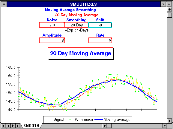
Depending on your monitor and graphics board, you may have to resize the window to see the entire worksheet. The chart shows the true trend line as a thin red line. This trend is masked by random variations from day to day, resulting in daily measurements drawn as green diamonds connected by yellow lines. The trend extracted by the selected moving average is drawn as a thick blue line. The closer the blue line approximates the red line indicating the true trend, the more effective the moving average has been in filtering out the short term random variations in the measurements.
You can control the moving average model by entering values in the following boxes of the control panel.
This parameter selects the type of moving average and its degree of smoothing. If positive, an exponentially smoothed moving average with smoothing constant equal to Smoothing is used. Only smoothing constants between 0 and 1 are valid. If negative, a simple moving average over the last -Smoothing days is used. To see the effects of a 20 day simple moving average, enter ``-20'' in the Smoothing cell.
The Noise value specifies the day to day random perturbation of
the basic trend. If you set Noise to 10, the measured values
will be randomly displaced ± 5 from the true trend. The random
displacement of points in the primary trend changes every time the
worksheet is recalculated. To show the effects of a different random
displacement of the current trend, press
![]() to force recalculation.
to force recalculation.
Since a moving average looks back at prior measurements, it lags the current trend. You can shift the moving average backward in time to cancel this lag by entering the number of days of displacement in the Shift cell. This allows you to compare the shape of the trend curve found by various moving averages with the original trend. A Shift value of zero disables displacement and produces a moving average that behaves, with respect to the actual trend, just as one calculated daily from current data. For a simple moving average, a Shift of half the days of Smoothing will generally align the trend and moving average. For an exponentially smoothed moving average, a Smoothing value of 0.9 can be aligned with a Shift of about 10.
The trend used in this model is generated by a cosine function. Amplitude controls the extent of the trend; the peak to peak variation is twice the value of Amplitude.
Rate controls the period of the primary trend, specified as the number of days from trough to peak and vice versa. As you decrease Rate, the trend varies more rapidly, requiring a shorter-term moving average to follow.
By John Walker