« September 2017 | Main | November 2017 »
Saturday, October 28, 2017
Floating Point Benchmark: Ruby Language Updated
I originally posted the results from a Ruby language version of my floating point benchmark on 2005-10-18. At that time, the current release of Ruby was version 1.8.3, and it performed toward the lower end of interpreted languages: at 26.1 times slower than C, slower than Python and Perl. In the twelve years since that posting, subsequent releases of Ruby have claimed substantial performance improvements, so I decided to re-run the test with the current stable version, 2.4.2p198, which I built from source code on my x86_64-linux development machine, as its Xubuntu distribution provides the older 2.3.1p112 release. Performance has, indeed, dramatically improved. I ran the benchmark for 21,215,057 iterations with a mean run time of 296.722 seconds for five runs, with a time per iteration of 13.9864 microseconds. The C benchmark on the same machine, built with GCC 5.4.0, runs at 1.7858 microseconds per iteration, so the current version of Ruby is now 7.832 times slower than C, making it one of the faster interpreted or byte coded languages. I have updated the language comparison result table in the FBENCH Web page to reflect these results. Here is the table as updated. I have also updated the Ruby version of the benchmark included in the archive to fix two warnings issued when the program was run with the -W2 option.| Language | Relative Time |
Details |
|---|---|---|
| C | 1 | GCC 3.2.3 -O3, Linux |
| JavaScript | 0.372 0.424 1.334 1.378 1.386 1.495 |
Mozilla Firefox 55.0.2, Linux Safari 11.0, MacOS X Brave 0.18.36, Linux Google Chrome 61.0.3163.91, Linux Chromium 60.0.3112.113, Linux Node.js v6.11.3, Linux |
| Chapel | 0.528 0.0314 |
Chapel 1.16.0, -fast, Linux Parallel, 64 threads |
| Visual Basic .NET | 0.866 | All optimisations, Windows XP |
| FORTRAN | 1.008 | GNU Fortran (g77) 3.2.3 -O3, Linux |
| Pascal | 1.027 1.077 |
Free Pascal 2.2.0 -O3, Linux GNU Pascal 2.1 (GCC 2.95.2) -O3, Linux |
| Swift | 1.054 | Swift 3.0.1, -O, Linux |
| Rust | 1.077 | Rust 0.13.0, --release, Linux |
| Java | 1.121 | Sun JDK 1.5.0_04-b05, Linux |
| Visual Basic 6 | 1.132 | All optimisations, Windows XP |
| Haskell | 1.223 | GHC 7.4.1-O2 -funbox-strict-fields, Linux |
| Scala | 1.263 | Scala 2.12.3, OpenJDK 9, Linux |
| Ada | 1.401 | GNAT/GCC 3.4.4 -O3, Linux |
| Go | 1.481 | Go version go1.1.1 linux/amd64, Linux |
| Simula | 2.099 | GNU Cim 5.1, GCC 4.8.1 -O2, Linux |
| Lua | 2.515 22.7 |
LuaJIT 2.0.3, Linux Lua 5.2.3, Linux |
| Python | 2.633 30.0 |
PyPy 2.2.1 (Python 2.7.3), Linux Python 2.7.6, Linux |
| Erlang | 3.663 9.335 |
Erlang/OTP 17, emulator 6.0, HiPE [native, {hipe, [o3]}] Byte code (BEAM), Linux |
| ALGOL 60 | 3.951 | MARST 2.7, GCC 4.8.1 -O3, Linux |
| PL/I | 5.667 | Iron Spring PL/I 0.9.9b beta, Linux |
| Lisp | 7.41 19.8 |
GNU Common Lisp 2.6.7, Compiled, Linux GNU Common Lisp 2.6.7, Interpreted |
| Smalltalk | 7.59 | GNU Smalltalk 2.3.5, Linux |
| Ruby | 7.832 | Ruby 2.4.2p198, Linux |
| Forth | 9.92 | Gforth 0.7.0, Linux |
| Prolog | 11.72 5.747 |
SWI-Prolog 7.6.0-rc2, Linux GNU Prolog 1.4.4, Linux, (limited iterations) |
| COBOL | 12.5 46.3 |
Micro Focus Visual COBOL 2010, Windows 7 Fixed decimal instead of computational-2 |
| Algol 68 | 15.2 | Algol 68 Genie 2.4.1 -O3, Linux |
| Perl | 23.6 | Perl v5.8.0, Linux |
| QBasic | 148.3 | MS-DOS QBasic 1.1, Windows XP Console |
| Mathematica | 391.6 | Mathematica 10.3.1.0, Raspberry Pi 3, Raspbian |
Posted at
00:11
![]()
Thursday, October 26, 2017
Floating Point Benchmark: Chapel Language Added
I have posted an update to my trigonometry-intense floating point benchmark which adds the Chapel language. Chapel (Cascade High Productivity Language) is a programming language developed by Cray, Inc. with the goal of integrating parallel computing into a language without cumbersome function calls or awkward syntax. The language implements both task based and data based parallelism: in the first, the programmer explicitly defines the tasks to be run in parallel, while in the second an operation is performed on a collection of data and the compiler and runtime system decides how to partition it among the computing resources available. Both symmetric multiprocessing with shared memory (as on contemporary “multi-core” microprocessors) and parallel architectures with local memory per processor and message passing are supported. Apart from its parallel processing capabilities, Chapel is a conventional object oriented imperative programming language. Programmers familiar with C++, Java, and other such languages will quickly become accustomed to its syntax and structure. Because this is the first parallel processing language in which the floating point benchmark has been implemented, I wanted to test its performance in both serial and parallel processing modes. Since the benchmark does not process large arrays of data, I used task parallelism to implement two kinds of parallel processing. The first is “parallel trace”, enabled by compiling with:chpl --fast fbench.chpl --set partrace=true
The ray tracing process propagates light of four different wavelengths through the lens assembly and then uses the object distance and axis slope angle of the rays to compute various aberrations. When partrace is set to true, the computation of these rays is performed in parallel, with four tasks running in a “cobegin” structure. When all of the tasks are complete, their results, stored in shared memory passed to the tasks by reference, is used to compute the aberrations. The second option is “parallel iteration”, enabled by compiling with:
chpl --fast fbench.chpl --set pariter=n
where n is the number of tasks among which the specified iteration count will be divided. On a multi-core machine, this should usually be set to the number of processor cores available, which you can determine on most Linux systems with:
cat /proc/cpuinfo | grep processor | wc -l
(If the number of tasks does not evenly divide the number of iterations, the extra iterations are assigned to one of the tasks.) The parallel iteration model might be seen as cheating, but in a number of applications, such as ray tracing for computer generated image rendering (as opposed to the ray tracing we do in the benchmark for optical design), a large number of computations are done which are independent of one another (for example, every pixel in a generated image is independent of every other), and the job can be parallelised by a simple “farm” algorithm which spreads the work over as many processors as are available. The parallel iteration model allows testing this approach with the floating point benchmark. If the benchmark is compiled without specifying partrace or pariter, it will run the task serially as in conventional language implementations. The number of iterations is specified on the command line when running the benchmark as:
./fbench --iterations=n
where n is the number to be run. After preliminary timing runs to determine the number of iterations, I ran the serial benchmark for 250,000,000 iterations, with run times in seconds of:
| user | real | sys | |
|---|---|---|---|
| 301.00 | 235.73 | 170.46 | |
| 299.24 | 234.26 | 169.27 | |
| 297.93 | 233.67 | 169.40 | |
| 301.02 | 236.05 | 171.08 | |
| 298.59 | 234.45 | 170.30 | |
| Mean | 299.56 | 234.83 | 170.10 |
    PR  NI    VIRT    RES    SHR S  %CPU %MEM     TIME+ COMMAND
    20   0  167900   2152   2012 S 199.7  0.0   0:12.54 fbench
Yup, almost 200% CPU utilisation. I then ran top -H to show
threads and saw:
    PR  NI    VIRT    RES    SHR S %CPU %MEM     TIME+ COMMAND
    20   0  167900   2152   2012 R 99.9  0.0   1:43.28 fbench
    20   0  167900   2152   2012 R 99.7  0.0   1:43.27 fbench
so indeed we had two threads. You can control the number of threads
with the environment variable CHPL_RT_NUM_THREADS_PER_LOCALE, so I
set:export CHPL_RT_NUM_THREADS_PER_LOCALE=1
and re-ran the benchmark, verifying with top that it was now using only one thread. I got the following times:
| user | real | sys | |
|---|---|---|---|
| 235.46 | 235.47 | 0.00 | |
| 236.52 | 236.55 | 0.02 | |
| 235.06 | 235.07 | 0.00 | |
| 235.17 | 235.20 | 0.02 | |
| 236.20 | 236.21 | 0.00 | |
| Mean | 235.68 |
| threads | real | user | sys |
|---|---|---|---|
| 1 | 16.92 | 16.91 | 0.00 |
| 2 | 30.74 | 41.68 | 18.16 |
| 4 | 43.15 | 68.23 | 90.65 |
| 5 | 64.29 | 112.38 | 358.88 |
| user | real | sys | |
|---|---|---|---|
| 342.27 | 48.95 | 39.84 | |
| 339.50 | 48.10 | 39.76 | |
| 343.01 | 49.34 | 42.19 | |
| 342.08 | 48.78 | 39.90 | |
| 338.83 | 47.70 | 37.30 | |
| Mean | 341.14 | 48.57 | 39.79 |
| threads | real | user | sys |
|---|---|---|---|
| 1 | 459.76 | 458.86 | 0.08 |
| 16 | 33.08 | 523.78 | 0.12 |
| 32 | 17.17 | 530.21 | 0.34 |
| 64 | 25.35 | 816.64 | 0.43 |
| threads | real | user | sys |
|---|---|---|---|
| 32 | 17.12 | 528.46 | 0.29 |
| 64 | 14.00 | 824.79 | 0.66 |
| Language | Relative Time |
Details |
|---|---|---|
| C | 1 | GCC 3.2.3 -O3, Linux |
| JavaScript | 0.372 0.424 1.334 1.378 1.386 1.495 |
Mozilla Firefox 55.0.2, Linux Safari 11.0, MacOS X Brave 0.18.36, Linux Google Chrome 61.0.3163.91, Linux Chromium 60.0.3112.113, Linux Node.js v6.11.3, Linux |
| Chapel | 0.528 0.0314 |
Chapel 1.16.0, -fast, Linux Parallel, 64 threads |
| Visual Basic .NET | 0.866 | All optimisations, Windows XP |
| FORTRAN | 1.008 | GNU Fortran (g77) 3.2.3 -O3, Linux |
| Pascal | 1.027 1.077 |
Free Pascal 2.2.0 -O3, Linux GNU Pascal 2.1 (GCC 2.95.2) -O3, Linux |
| Swift | 1.054 | Swift 3.0.1, -O, Linux |
| Rust | 1.077 | Rust 0.13.0, --release, Linux |
| Java | 1.121 | Sun JDK 1.5.0_04-b05, Linux |
| Visual Basic 6 | 1.132 | All optimisations, Windows XP |
| Haskell | 1.223 | GHC 7.4.1-O2 -funbox-strict-fields, Linux |
| Scala | 1.263 | Scala 2.12.3, OpenJDK 9, Linux |
| Ada | 1.401 | GNAT/GCC 3.4.4 -O3, Linux |
| Go | 1.481 | Go version go1.1.1 linux/amd64, Linux |
| Simula | 2.099 | GNU Cim 5.1, GCC 4.8.1 -O2, Linux |
| Lua | 2.515 22.7 |
LuaJIT 2.0.3, Linux Lua 5.2.3, Linux |
| Python | 2.633 30.0 |
PyPy 2.2.1 (Python 2.7.3), Linux Python 2.7.6, Linux |
| Erlang | 3.663 9.335 |
Erlang/OTP 17, emulator 6.0, HiPE [native, {hipe, [o3]}] Byte code (BEAM), Linux |
| ALGOL 60 | 3.951 | MARST 2.7, GCC 4.8.1 -O3, Linux |
| PL/I | 5.667 | Iron Spring PL/I 0.9.9b beta, Linux |
| Lisp | 7.41 19.8 |
GNU Common Lisp 2.6.7, Compiled, Linux GNU Common Lisp 2.6.7, Interpreted |
| Smalltalk | 7.59 | GNU Smalltalk 2.3.5, Linux |
| Forth | 9.92 | Gforth 0.7.0, Linux |
| Prolog | 11.72 5.747 |
SWI-Prolog 7.6.0-rc2, Linux GNU Prolog 1.4.4, Linux, (limited iterations) |
| COBOL | 12.5 46.3 |
Micro Focus Visual COBOL 2010, Windows 7 Fixed decimal instead of computational-2 |
| Algol 68 | 15.2 | Algol 68 Genie 2.4.1 -O3, Linux |
| Perl | 23.6 | Perl v5.8.0, Linux |
| Ruby | 26.1 | Ruby 1.8.3, Linux |
| QBasic | 148.3 | MS-DOS QBasic 1.1, Windows XP Console |
| Mathematica | 391.6 | Mathematica 10.3.1.0, Raspberry Pi 3, Raspbian |
Posted at
21:41
![]()
Monday, October 23, 2017
ISBNiser 1.3 Update Released
I have just posted version 1.3 of ISBNiser, a utility for validating publication numbers in the ISBN-13 and ISBN-10 formats, converting between the formats, and generating Amazon associate links to purchase items with credit to a specified account. Version 1.3 adds the ability to automatically parse the specified ISBNs and insert delimiters among the elements (unique country code [ISBN-13 only], registration group, registrant, publication, and checksum). If the number supplied contains delimiters, the same delimiter (the first if multiple different delimiters appear) will be used when re-generating the number with delimiters. For example, if all the publisher gives you is “9781481487658”, you can obtain an ISBN-13 or ISBN-10 with proper delimiters with:$ isbniser 9781481487658 ISBN-13: 978-1-4814-8765-8 9781481487658 ISBN-10: 1481487655 1-4814-8765-5The rules for properly placing the delimiters in an ISBN are deliciously baroque, with every language and country group having their own way of going about it. ISBNiser implements this standard with a page of ugly code. If confronted with an ISBN that does not conform to the standard (I haven't yet encountered one, but in the wild and wooly world of international publishing it wouldn't surprise me), it issues a warning message and returns a number with no delimiters. If the “−p” option is specified, delimiters in the number given will be preserved, regardless of where they are placed. When the “−n” option is specified, allowing invalid ISBN specifications (for example, when generating links to products on Amazon with ASIN designations), no attempt to insert delimiters is made.
Posted at
14:13
![]()
Sunday, October 22, 2017
New: Commodore Curiosities
In the late 1980s I became interested in mass market home computers as possible markets for some products I was considering developing. I bought a Commodore 128 and began to experiment with it, writing several programs, some of which were published in Commodore user magazines. Commodore Curiosities presents three of those programs: a customisable key click generator, a moon phase calculator, and a neural network simulator. Complete source code and a floppy disc image which can be run on modern machines under the VICE C-64/C-128 emulator is included for each program.Posted at
19:50
![]()
Wednesday, October 18, 2017
WatchFull Updated
WatchFull is a collection of programs, written in Perl, which assist Unix systems administrators in avoiding and responding to file system space exhaustion crises. WatchFull monitors file systems and reports when they fall below a specified percentage of free space. LogJam watches system and application log files (for example Web server access and error logs) and warns when they exceed a threshold size. Top40 scans a file system or directory tree and provides a list of the largest files within it. I have just posted the first update to WatchFull since its initial release in 2000. Version 1.1 updates the source code to current Perl syntax, corrects several warning messages, and now runs in “use strict;” and “use warnings;” modes. The source code should be compatible with any recent version of Perl 5. The HTML documentation has been updated to XHTML 1.0 Strict, CSS3, and Unicode typography. WatchFull Home PagePosted at
19:55
![]()
Monday, October 16, 2017
New: Marinchip Systems: Documents and Images
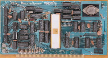 I have just posted an archive of documents and images about Marinchip Systems, the company I founded and operated from 1977 through 1985. Marinchip delivered, starting in 1978, the first true 16-bit personal computer on the S-100 bus, with the goal of providing its users the same experience as conecting to a commercial timesharing service which cost many times more. While other personal computer companies were providing 8 Kb BASIC, we had a Unix-like operating system, Pascal, and eventually a multi-user system.
Marinchip (which was named after the Marinship shipyard not far from where I lived, which made Liberty ships during World War II), designed its own hardware and software, with hardware based upon the Texas Instruments TMS9900 microprocessor and the software written by, well, me.
Texas Instruments (TI) in this era was a quintessential engineering company: “Hey, we've designed something cool. Let's go design something else, entirely different, which is even cooler!” There didn't seem to be anybody who said, “No, first you need to offer follow-on products which allow those who bet on your original product to evolve and grow as technology advances.” TI built a supercomputer, the TI-ASC, at the time one of the fastest in the world, but then they lost interest in it and sold only seven.
The Marinchip 9900 did somewhat better, although its performance and unit cost were more modest. Hughes Radar Systems designed our board into the F-16 radar tester and bought the boards in large quantities for this embedded application. The 9900 processor was one of the only 16-bit processors qualified for use in geosynchronous satellites, and we sold a number of systems to satellite manufacturers for software development because our systems cost a fraction of those sold by Texas Instruments. In 1985, after Autodesk took off, and I had no more time for Marinchip, I sold the company, with all of its hardware, software, and manufacturing rights to Hughes Electronics which had, by then, been acquired by General Motors, so I said, “I sold my company to General Motors”.
I have just posted an archive of documents and images about Marinchip Systems, the company I founded and operated from 1977 through 1985. Marinchip delivered, starting in 1978, the first true 16-bit personal computer on the S-100 bus, with the goal of providing its users the same experience as conecting to a commercial timesharing service which cost many times more. While other personal computer companies were providing 8 Kb BASIC, we had a Unix-like operating system, Pascal, and eventually a multi-user system.
Marinchip (which was named after the Marinship shipyard not far from where I lived, which made Liberty ships during World War II), designed its own hardware and software, with hardware based upon the Texas Instruments TMS9900 microprocessor and the software written by, well, me.
Texas Instruments (TI) in this era was a quintessential engineering company: “Hey, we've designed something cool. Let's go design something else, entirely different, which is even cooler!” There didn't seem to be anybody who said, “No, first you need to offer follow-on products which allow those who bet on your original product to evolve and grow as technology advances.” TI built a supercomputer, the TI-ASC, at the time one of the fastest in the world, but then they lost interest in it and sold only seven.
The Marinchip 9900 did somewhat better, although its performance and unit cost were more modest. Hughes Radar Systems designed our board into the F-16 radar tester and bought the boards in large quantities for this embedded application. The 9900 processor was one of the only 16-bit processors qualified for use in geosynchronous satellites, and we sold a number of systems to satellite manufacturers for software development because our systems cost a fraction of those sold by Texas Instruments. In 1985, after Autodesk took off, and I had no more time for Marinchip, I sold the company, with all of its hardware, software, and manufacturing rights to Hughes Electronics which had, by then, been acquired by General Motors, so I said, “I sold my company to General Motors”.
What can you learn from this? Probably not a heck of a lot. Certainly, I learned little. I repeated most of my mistakes from Marinchip in Autodesk, and only learned later, from experience, that there are things which work at one scale which don't when the numbers are ten or a hundred times larger. Still, if you haven't seen personal computing as it existed while Jimmy Carter was the U.S. president, take a glance. As far as I know, nothing we did at Marinchip contributed in any way to our current technology. Well, almost nothing. There was this curious drafting program one of our customers developed which was the inspiration for AutoCAD…. Marinchip Systems: Documents and Images
Posted at
19:15
![]()
Wednesday, October 11, 2017
Reading List: The Planet Remade
- Morton, Oliver. The Planet Remade. Princeton: Princeton University Press, 2015. ISBN 978-0-691-17590-4.
-
We live in a profoundly unnatural world. Since the start of the
industrial revolution, and rapidly accelerating throughout the
twentieth century, the actions of humans have begun to influence
the flow of energy and materials in the Earth's biosphere on a
global scale. Earth's current human population and standard of
living are made possible entirely by industrial production of
nitrogen-based fertilisers and crop plants bred to efficiently
exploit them. Industrial production of fixed (chemically
reactive) nitrogen from the atmosphere now substantially exceeds
all of that produced by the natural soil bacteria on the planet
which, prior to 1950, accounted for almost all of the nitrogen
required to grow plants. Fixing nitrogen by the Haber-Bosch
process is energy-intensive, and consumes around 1.5 percent
of all the world's energy usage and, as a feedstock, 3–5%
of natural gas produced worldwide. When we eat these crops, or
animals fed from them, we are, in a sense, eating fossil fuels.
On the order of four out of five nitrogen molecules that make up
your body were made in a factory by the Haber-Bosch process. We
are the children, not of nature, but of industry.
The industrial production of fertiliser, along with crops
tailored to use them, is entirely responsible for the rapid
growth of the Earth's population, which has increased from around
2.5 billion in 1950, when industrial fertiliser and
“green revolution” crops came into wide use, to
more than 7 billion today. This was accompanied not by the collapse
into global penury predicted by Malthusian doom-sayers,
but rather a broad-based rise in the standard of living, with
extreme poverty and malnutrition falling to all-time
historical lows. In the lifetimes of many people, including
this scribbler, our species has taken over the flow of nitrogen
through the Earth's biosphere, replacing a process mediated by
bacteria for billions of years with one performed in factories.
The flow of nitrogen from atmosphere to soil, to plants and
the creatures who eat them, back to soil, sea, and ultimately
the atmosphere is now largely in the hands of humans, and
their very lives have become dependent upon it.
This is an example of “geoengineering”—taking
control of what was a natural process and replacing it with
an engineered one to produce a desired outcome: in this case,
the ability to feed a much larger population with an
unprecedented standard of living. In the case of nitrogen
fixation, there wasn't a grand plan drawn up to do all of this:
each step made economic sense to the players involved. (In fact,
one of the motivations for developing the Haber-Bosch process was
not to produce fertiliser, but rather to produce feedstocks for
the manufacture of military and industrial explosives, which had
become dependent on nitrates obtained from guano imported to
Europe from South America.) But the outcome was the same: ours
is an engineered world. Those who are repelled by such an
intervention in natural processes or who are concerned by
possible detrimental consequences of it, foreseen or
unanticipated, must come to terms with the reality that
abandoning this world-changing technology now would result in
the collapse of the human population, with at least half of
the people alive today starving to death, and many of the
survivors reduced to subsistence in abject poverty. Sadly, one
encounters fanatic “greens” who think this would be
just fine (and, doubtless, imagining they'd be among the
survivors).
Just mentioning geoengineering—human intervention and
management of previously natural processes on a global
scale—may summon in the minds of many Strangelove-like
technological megalomania or the hubris of Bond villains,
so it's important to bear in mind that we're already
doing it, and have become utterly dependent upon it.
When we consider the challenges we face in accommodating
a population which is expected to grow to ten billion by
mid-century (and, absent catastrophe, this is almost a
given: the parents of the ten billion are mostly alive
today), who will demand and deserve a standard of living
comparable to what they see in industrial economies, and
while carefully weighing the risks and uncertainties involved,
it may be unwise to rule out other geoengineering interventions
to mitigate undesirable consequences of supporting the
human population.
In parallel with the human takeover of the nitrogen cycle,
another geoengineering project has been underway, also
rapidly accelerating in the 20th century, driven both by
population growth and industrialisation of previously
agrarian societies. For hundreds of millions of years, the Earth
also cycled carbon through the atmosphere, oceans, biosphere,
and lithosphere. Carbon dioxide (CO₂) was metabolised
from the atmosphere by photosynthetic plants, extracting carbon for their
organic molecules and producing oxygen released to the atmosphere, then
passed along as plants were eaten, returned to the soil,
or dissolved in the oceans, where creatures incorporated
carbonates into their shells, which eventually became limestone
rock and, over geological time, was subducted as the
continents drifted, reprocessed far below the surface, and
expelled back into the atmosphere by volcanoes. (This is a
gross oversimplification of the
carbon cycle,
but we don't need to go further into it for what follows. The
point is that it's something which occurs on a time scale of
tens to hundreds of millions of years and on which humans, prior
to the twentieth century, had little influence.)
The natural carbon cycle is not leakproof. Only part of the
carbon sequestered by marine organisms and immured in limestone
is recycled by volcanoes; it is estimated that this loss of
carbon will bring the era of multicellular life on Earth to an
end around a billion years from now. The carbon in some plants
is not returned to the biosphere when they die. Sometimes, the
dead vegetation accumulates in dense beds where it is protected
against oxidation and eventually forms deposits of peat, coal,
petroleum, and natural gas. Other than natural seeps and
releases of the latter substances, their carbon is also largely
removed from the biosphere. Or at least it was until those
talking apes came along….
The modern technological age has been powered by the exploitation of these fossil fuels: laid down over hundreds of millions of years, often under special conditions which only existed in certain geological epochs, in the twentieth century their consumption exploded, powering our present technological civilisation. For all of human history up to around 1850, world energy consumption was less than 20 exajoules per year, almost all from burning biomass such as wood. (What's an exajoule? Well, it's 1018 joules, which probably tells you absolutely nothing. That's a lot of energy: equivalent to 164 million barrels of oil, or the capacity of around sixty supertankers. But it's small compared to the energy the Earth receives from the Sun, which is around 4 million exajoules per year.) By 1900, the burning of coal had increased this number to 33 exajoules, and this continued to grow slowly until around 1950 when, with oil and natural gas coming into the mix, energy consumption approached 100 exajoules. Then it really took off. By the year 2000, consumption was 400 exajoules, more than 85% from fossil fuels, and today it's more than 550 exajoules per year.
Now, as with the nitrogen revolution, nobody thought about this as geoengineering, but that's what it was. Humans were digging up, or pumping out, or otherwise tapping carbon-rich substances laid down long before their clever species evolved and burning them to release energy banked by the biosystem from sunlight in ages beyond memory. This is a human intervention into the Earth's carbon cycle of a magnitude even greater than the Haber-Bosch process into the nitrogen cycle. “Look out, they're geoengineering again!” When you burn fossil fuels, the combustion products are mostly carbon dioxide and water. There are other trace products, such as ash from coal, oxides of nitrogen, and sulphur compounds, but other than side effects such as various forms of pollution, they don't have much impact on the Earth's recycling of elements. The water vapour from combustion is rapidly recycled by the biosphere and has little impact, but what about the CO₂? Well, that's interesting. CO₂ is a trace gas in the atmosphere (less than a fiftieth of a percent), but it isn't very reactive and hence doesn't get broken down by chemical processes. Once emitted into the atmosphere, CO₂ tends to stay there until it's removed via photosynthesis by plants, weathering of rocks, or being dissolved in the ocean and used by marine organisms. Photosynthesis is an efficient consumer of atmospheric carbon dioxide: a field of growing maize in full sunlight consumes all of the CO₂ within a metre of the ground every five minutes—it's only convection that keeps it growing. You can see the yearly cycle of vegetation growth in measurements of CO₂ in the atmosphere as plants take it up as they grow and then release it after they die. The other two processes are much slower. An increase in the amount of CO₂ causes plants to grow faster (operators of greenhouses routinely enrich their atmosphere with CO₂ to promote growth), and increases the root to shoot ratio of the plants, tending to remove CO₂ from the atmosphere where it will be recycled more slowly into the biosphere. But since the start of the industrial revolution, and especially after 1950, the emission of CO₂ by human activity over a time scale negligible on the geological scale by burning of fossil fuels has released a quantity of carbon into the atmosphere far beyond the ability of natural processes to recycle. For the last half billion years, the CO₂ concentration in the atmosphere has varied between 280 parts per million in interglacial (warm periods) and 180 parts per million during the depths of the ice ages. The pattern is fairly consistent: a rapid rise of CO₂ at the end of an ice age, then a slow decline into the next ice age. The Earth's temperature and CO₂ concentrations are known with reasonable precision in such deep time due to ice cores taken in Greenland and Antarctica, from which temperature and atmospheric composition can be determined from isotope ratios and trapped bubbles of ancient air. While there is a strong correlation between CO₂ concentration and temperature, this doesn't imply causation: the CO₂ may affect the temperature; the temperature may affect the CO₂; they both may be caused by another factor; or the relationship may be even more complicated (which is the way to bet). But what is indisputable is that, as a result of our burning of all of that ancient carbon, we are now in an unprecedented era or, if you like, a New Age. Atmospheric CO₂ is now around 410 parts per million, which is a value not seen in the last half billion years, and it's rising at a rate of 2 parts per million every year, and accelerating as global use of fossil fuels increases. This is a situation which, in the ecosystem, is not only unique in the human experience; it's something which has never happened since the emergence of complex multicellular life in the Cambrian explosion. What does it all mean? What are the consequences? And what, if anything, should we do about it? (Up to this point in this essay, I believe everything I've written is non-controversial and based upon easily-verified facts. Now we depart into matters more speculative, where squishier science such as climate models comes into play. I'm well aware that people have strong opinions about these issues, and I'll not only try to be fair, but I'll try to stay away from taking a position. This isn't to avoid controversy, but because I am a complete agnostic on these matters—I don't think we can either measure the raw data or trust our computer models sufficiently to base policy decisions upon them, especially decisions which might affect the lives of billions of people. But I do believe that we ought to consider the armanentarium of possible responses to the changes we have wrought, and will continue to make, in the Earth's ecosystem, and not reject them out of hand because they bear scary monikers like “geoengineering”.) We have been increasing the fraction of CO₂ in the atmosphere to levels unseen in the history of complex terrestrial life. What can we expect to happen? We know some things pretty well. Plants will grow more rapidly, and many will produce more roots than shoots, and hence tend to return carbon to the soil (although if the roots are ploughed up, it will go back to the atmosphere). The increase in CO₂ to date will have no physiological effects on humans: people who work in greenhouses enriched to up to 1000 parts per million experience no deleterious consequences, and this is more than twice the current fraction in the Earth's atmosphere, and at the current rate of growth, won't be reached for three centuries. The greatest consequence of a growing CO₂ concentration is on the Earth's energy budget. The Earth receives around 1360 watts per square metre on the side facing the Sun. Some of this is immediately reflected back to space (much more from clouds and ice than from land and sea), and the rest is absorbed, processed through the Earth's weather and biosphere, and ultimately radiated back to space at infrared wavelengths. The books balance: the energy absorbed by the Earth from the Sun and that it radiates away are equal. (Other sources of energy on the Earth, such as geothermal energy from radioactive decay of heavy elements in the Earth's core and energy released by human activity are negligible at this scale.) Energy which reaches the Earth's surface tends to be radiated back to space in the infrared, but some of this is absorbed by the atmosphere, in particular by trace gases such as water vapour and CO₂. This raises the temperature of the Earth: the so-called greenhouse effect. The books still balance, but because the temperature of the Earth has risen, it emits more energy. (Due to the Stefan-Boltzmann law, the energy emitted from a black body rises as the fourth power of its temperature, so it doesn't take a large increase in temperature [measured in degrees Kelvin] to radiate away the extra energy.) So, since CO₂ is a strong absorber in the infrared, we should expect it to be a greenhouse gas which will raise the temperature of the Earth. But wait—it's a lot more complicated. Consider: water vapour is a far greater contributor to the Earth's greenhouse effect than CO₂. As the Earth's temperature rises, there is more evaporation of water from the oceans and lakes and rivers on the continents, which amplifies the greenhouse contribution of the CO₂. But all of that water, released into the atmosphere, forms clouds which increase the albedo (reflectivity) of the Earth, and reduce the amount of solar radiation it absorbs. How does all of this interact? Well, that's where the global climate models get into the act, and everything becomes very fuzzy in a vast panel of twiddle knobs, all of which interact with one another and few of which are based upon unambiguous measurements of the climate system. Let's assume, arguendo, that the net effect of the increase in atmospheric CO₂ is an increase in the mean temperature of the Earth: the dreaded “global warming”. What shall we do? The usual prescriptions, from the usual globalist suspects, are remarkably similar to their recommendations for everything else which causes their brows to furrow: more taxes, less freedom, slower growth, forfeit of the aspirations of people in developing countries for the lifestyle they see on their smartphones of the people who got to the industrial age a century before them, and technocratic rule of the masses by their unelected self-styled betters in cheap suits from their tawdry cubicle farms of mediocrity. Now there's something to stir the souls of mankind! But maybe there's an alternative. We've already been doing geoengineering since we began to dig up coal and deploy the steam engine. Maybe we should embrace it, rather than recoil in fear. Suppose we're faced with global warming as a consequence of our inarguable increase in atmospheric CO₂ and we conclude its effects are deleterious? (That conclusion is far from obvious: in recorded human history, the Earth has been both warmer and colder than its present mean temperature. There's an intriguing correlation between warm periods and great civilisations versus cold periods and stagnation and dark ages.) How might we respond? Atmospheric veil. Volcanic eruptions which inject large quantities of particulates into the stratosphere have been directly shown to cool the Earth. A small fleet of high-altitude airplanes injecting sulphate compounds into the stratosphere would increase the albedo of the Earth and reflect sufficient sunlight to reduce or even cancel or reverse the effects of global warming. The cost of such a programme would be affordable by a benevolent tech billionaire or wannabe Bond benefactor (“Greenfinger”), and could be implemented in a couple of years. The effect of the veil project would be much less than a volcanic eruption, and would be imperceptible other than making sunsets a bit more colourful. Marine cloud brightening. By injecting finely-dispersed salt water from the ocean into the atmosphere, nucleation sites would augment the reflectivity of low clouds above the ocean, increasing the reflectivity (albedo) of the Earth. This could be accomplished by a fleet of low-tech ships, and could be applied locally, for example to influence weather. Carbon sequestration. What about taking the carbon dioxide out of the atmosphere? This sounds like a great idea, and appeals to clueless philanthropists like Bill Gates who are ignorant of thermodynamics, but taking out a trace gas is really difficult and expensive. The best place to capture it is where it's densest, such as the flue of a power plant, where it's around 10%. The technology to do this, “carbon capture and sequestration” (CCS) exists, but has not yet been deployed on any full-scale power plant. Fertilising the oceans. One of the greatest reservoirs of carbon is the ocean, and once carbon is incorporated into marine organisms, it is removed from the biosphere for tens to hundreds of millions of years. What constrains how fast critters in the ocean can take up carbon dioxide from the atmosphere and turn it into shells and skeletons? It's iron, which is rare in the oceans. A calculation made in the 1990s suggested that if you added one tonne of iron to the ocean, the bloom of organisms it would spawn would suck a hundred thousand tonnes of carbon out of the atmosphere. Now, that's leverage which would impress even the most jaded Wall Street trader. Subsequent experiments found the ratio to be maybe a hundred times less, but then iron is cheap and it doesn't cost much to dump it from ships. Great Mambo Chicken. All of the previous interventions are modest, feasible with existing technology, capable of being implemented incrementally while monitoring their effects on the climate, and easily and quickly reversed should they be found to have unintended detrimental consequences. But when thinking about affecting something on the scale of the climate of a planet, there's a tendency to think big, and a number of grand scale schemes have been proposed, including deploying giant sunshades, mirrors, or diffraction gratings at the L1 Lagrangian point between the Earth and the Sun. All of these would directly reduce the solar radiation reaching the Earth, and could be adjusted as required to manage the Earth's mean temperature at any desired level regardless of the composition of its atmosphere. Such mega-engineering projects are considered financially infeasible, but if the cost of space transportation falls dramatically in the future, might become increasingly attractive. It's worth observing that the cost estimates for such alternatives, albeit in the tens of billions of dollars, are small compared to re-architecting the entire energy infrastructure of every economy in the world to eliminate carbon-based fuels, as proposed by some glib and innumerate environmentalists. We live in the age of geoengineering, whether we like it or not. Ever since we started to dig up coal and especially since we took over the nitrogen cycle of the Earth, human action has been dominant in the Earth's ecosystem. As we cope with the consequences of that human action, we shouldn't recoil from active interventions which acknowledge that our environment is already human-engineered, and that it is incumbent upon us to preserve and protect it for our descendants. Some environmentalists oppose any form of geoengineering because they feel it is unnatural and provides an alternative to restoring the Earth to an imagined pre-industrial pastoral utopia, or because it may be seized upon as an alternative to their favoured solutions such as vast fields of unsightly bird shredders. But as David Deutsch says in The Beginning of Infinity, “Problems are inevitable“; but “Problems are soluble.” It is inevitable that the large scale geoengineering which is the foundation of our developed society—taking over the Earth's natural carbon and nitrogen cycles—will cause problems. But it is not only unrealistic but foolish to imagine these problems can be solved by abandoning these pillars of modern life and returning to a “sustainable” (in other words, medieval) standard of living and population. Instead, we should get to work solving the problems we've created, employing every tool at our disposal, including new sources of energy, better means of transmitting and storing energy, and geoengineering to mitigate the consequences of our existing technologies as we incrementally transition to those of the future.
Posted at
13:35
![]()
Tuesday, October 10, 2017
New: ISBNiser Utility
As I read and review lots of books, I frequently need to deal with International Standard Book Numbers (ISBNs) which, like many international standards, come in a rainbow of flavours, all confusing and some distasteful. There are old ISBN-10s, new ISBN-13s, the curious way in which ISBN-13s were integrated into EANs, “Bookland”, and its two islands, 978 legacy, which maps into ISBN-10, and 979, sparsely populated, which doesn't. Of course, these important numbers, which have been central to commerce in books since the 1970s and to Internet booksellers today, contain a check digit to guard against transcription and transposition errors and, naturally, the two flavours, ISBN-10 and ISBN-13 use entirely different algorithms to compute it, with the former working in base eleven, which even those of us who endured “new math” in the 1960s managed to evade. I've just published ISBNiser, a cleaned-up version of a program I've been using in house since 2008 to cope with all of this. It validates ISBNs in both the 10- and 13-digit formats, interconverts between them, and generates links to purchase the book cited at Amazon, on any Amazon national site, and optionally credits the purchase to your Amazon Associates account or an alternative account you can specify when configuring the program. You can specify ISBNs with or without delimiters among the digits, and with any (non-alphanumeric) delimiter you wish. If you're faced with an all-numeric ISBN as is becoming more common as publishers move down-market, you can put the hyphens back with the U.S. Library of Congress ISBN Converter, which will give you an ISBN-10 you can convert back to ISBN-13 with ISBNiser. ISBNiser Home PagePosted at
23:09
![]()
Sunday, October 8, 2017
The Hacker's Diet Online: Source Code Release Update
The Hacker's Diet Online has been in production at Fourmilab since July, 2007: more than ten years. It provides, in a Web application which can be accessed from any browser or mobile device with Web connectivity, a set of tools for planning, monitoring, and analysing the progress of a diet and subsequently maintaining a stable weight as described in my 1991 book The Hacker's Diet. The application was originally hosted on Fourmilab's local server farm, but as of January, 2016, Fourmilab's Web site has been hosted on Amazon Web Services (AWS). Due to changes in the server environment, a few modifications had to be made to the application, none of which are visible to the user. These changes were applied as “hot fixes” to the running code, and not integrated back into the master source code, which is maintained using the Literate Programming tool Nuweb. I have just completed this integration and posted an updated version of the published program (1.4 Mb PDF) and downloadable source code (2.7 Mb tar.gz). The code generated from this program is identical to that running on the server, with the exception of passwords, encryption keys, and other security-related information which have been changed for the obvious reasons. A complete list of the changes in this release appears in the change log at the end of the published program. The Hacker's Diet Online now has more than 30,000 open accounts, not counting completely inactive accounts which never posted any data after being opened, which are archived and purged every few years.Posted at
20:14
![]()
Monday, October 2, 2017
Floating Point Benchmark: JavaScript Language Updated
I have posted an update to my trigonometry-intense floating point benchmark which updates the benchmarks for JavaScript, last run in 2005. A new release of the benchmark collection including the updated JavaScript benchmark is now available for downloading. This JavaScript benchmark was originally developed in 2005 and browser timing tests were run in 2005 and 2006. At the time, most implementations of JavaScript were pure interpreters or interpreters of a byte-code representation, and their performance reflected this. With the run time of the C benchmark taken as 1, JavaScript ran anywhere from 27.6 (Opera 8.0) to 46.9 (Mozilla Firefox 1.0.6) times slower. What a difference a decade makes! The JavaScript engines in the leading modern browsers use optimisation and techniques such as just-in-time compilation to deliver performance which is often competitive with languages that compile to machine code. This is what permitted me to re-implement Cellular Automata Laboratory as an application which ran entirely within the browser, eliminating the need for a separate programming language environment. Having observed how well JavaScript performed in that project, it was clear that the time had come to revisit the language and compare contemporary implementations with C. The benchmark is essentially unchanged from the one run in 2005. I have added some declarations of variables to make the code compliant with "use strict", added some comments to the code, and included a main program which allows the benchmark to run from the command line under node.js, but there are no changes to the code which is timed when running the benchmark. Comparisons to the execution time of the C benchmark were made against a version compiled with GCC 5.4.0. A recent release of the mathematical function library for GCC appears to have dramatically slowed down the trigonometric functions, apparently in the interest of last-bit accuracy, perhaps by as much as a factor of two compared to previous libraries. That should be kept in mind when considering the comparisons with JavaScript implementations. The change to the C library trigonometric functions made no difference in the results computed by the benchmark, which are verified to 13 significant digits. A variety of JavaScript engines are used by current browsers. One would expect that performance in a JavaScript benchmark among browsers which share the same engine would be about the same, and the results confirm this. There are, however, dramatic differences among engines. For each JavaScript implementation, I ran the benchmark five times on an idle machine, using an iteration count calculated to result in a run time of approximately five minutes. I then computed the mean time of the five runs and divided by the iteration count to obtain the run time in microseconds per iteration. As the reference, I started with the C version, compiled with GCC 5.4.0, and run for 166,051,660 iterations. Run times in seconds were (296.89, 296.37, 296.29, 296.76, 296.37) for a mean time of 296.536, or 1.7858 microseconds per iteration. The first test I ran was with Node.js v6.11.3. This is a command line environment which uses the V8 JavaScript engine also used by Google Chrome. I ran 112,697,692 iterations and measured run times in seconds of (300.001, 300.542, 300.850, 301.022, 302.053) with a mean of 300.8936, and 2.6699 microseconds per iteration. This is 1.4951 times slower than C. Next was Google Chrome version 61.0.3163.91, which was run for 119,019,281 iterations with timings of (293.573, 293.420, 292.188, 292.740, 292.939) with a mean of 292.972 seconds and 2.4616 microseconds per iteration, which is 1.3784 times slower than C. I then tested Chromium, the free version of the browser upon which Google Chrome is built, version 60.0.3112.113, and as expected, the results were almost identical: 1.3863 times slower than C. The Brave browser is derived from the Chromium code base and thus inherits its V8 JavaScript engine. Version 0.18.36 was a little bit faster in the tests, coming in at 1.3336 times slower than C. So far, the results were pretty much consistent with what I'd observed during the Cellular Automata Laboratory project: JavaScript performs at a speed competitive to compiled languages or the better byte code languages, and is suitable for all but the most computationally-intense tasks. Next up was Mozilla Firefox, which was now on version 55.0.2, a long way from the 1.0.6 I tested in 2005. Firefox uses its own JavaScript engine called Rhino, which is written in Java and compiles JavaScript into Java bytecode, which is executed with a just-in-time compiler. When I ran the benchmark, I could scarcely believe my eyes. I had to use an iteration count of 457,577,013 (yes, nearly half a billion) to achieve a run time around five minutes. I measured run times of (303.958, 303.255, 303.683, 304.136, 304.283) seconds with a mean of 393.863, or 0.6641 microseconds per iteration. This is simply stunning: the ratio of run time to C is 0.3719 or, taking the reciprocal, JavaScript in Firefox ran the benchmark almost 2.7 times faster than C, compiled with GCC to native 64-bit Intel machine code in full optimising mode. What's going on here? My guess is that we're seeing the poor performance of the new GCC trigonometric function libraries taking their toll. Fbench is far more intense in its use of trigonometric functions than even most other scientific software, so a slow implementation of these functions will show up strongly in the results. I suspect the Java engine which ultimately runs the JavaScript code of the benchmark uses different libraries which, although perhaps less accurate (but entirely adequate for this program), run much faster than those now used by GCC. The final test was a little bit more involved, since it tested Apple's Safari browser which uses a JavaScript engine called Nitro that is part of the WebKit framework. Current releases incorporate just-in-time compilation to machine code. In order to time this browser, I had to run it on a Macintosh Pro instead of the Dell laptop running Xubuntu Linux on which all the other tests were run. The Macintosh dates from 2008, and is substantially slower than the Dell machine. To adjust results to compensate for this speed difference, I ran the Perl version of the benchmark on the two machines and divided the run times to obtain the speed ratio between them. Since the Perl benchmark was identical and the two machines were running comparable versions of Perl, this provides a reasonable estimate of their relative performance. Running the benchmark in Safari 11.0 (11604.1.38.1.7), it immediately became clear this was another fast one. I needed an iteration count of 177,542,107 to obtain the desired run time of around five minutes, and I measured the following times: (299.428, 299.418, 299.417, 299.439, 299.400) for a mean of 299.4204 seconds and 1.6865 microseconds per iteration. But since this machine is less than half the speed of the Dell, this must be multiplied by the speed ratio of 0.4487 to obtain an equivalent time of 0.7567 microseconds per iteration had the Macintosh been as fast as the machine on which the other benchmarks were run. This works out to a run time ratio of 0.4237 compared to C, or about 2.36 times faster than C; in the same ballpark as Firefox and much faster than the V8-based systems. Here is a table summarising the results, ranked from fastest to slowest.| Browser/System | JavaScript Engine | Run Time vs. C |
|---|---|---|
| Mozilla Firefox | Rhino | 0.3719 |
| Safari (Mac OS X) | Nitro | 0.4237 |
| Brave | V8 | 1.3336 |
| Google Chrome | V8 | 1.3784 |
| Chromium | V8 | 1.3863 |
| Node.js | V8 | 1.4951 |
| Language | Relative Time |
Details |
|---|---|---|
| C | 1 | GCC 3.2.3 -O3, Linux |
| JavaScript | 0.372 0.424 1.334 1.378 1.386 1.495 |
Mozilla Firefox 55.0.2, Linux Safari 11.0, MacOS X Brave 0.18.36, Linux Google Chrome 61.0.3163.91, Linux Chromium 60.0.3112.113, Linux Node.js v6.11.3, Linux |
| Visual Basic .NET | 0.866 | All optimisations, Windows XP |
| FORTRAN | 1.008 | GNU Fortran (g77) 3.2.3 -O3, Linux |
| Pascal | 1.027 1.077 |
Free Pascal 2.2.0 -O3, Linux GNU Pascal 2.1 (GCC 2.95.2) -O3, Linux |
| Swift | 1.054 | Swift 3.0.1, -O, Linux |
| Rust | 1.077 | Rust 0.13.0, --release, Linux |
| Java | 1.121 | Sun JDK 1.5.0_04-b05, Linux |
| Visual Basic 6 | 1.132 | All optimisations, Windows XP |
| Haskell | 1.223 | GHC 7.4.1-O2 -funbox-strict-fields, Linux |
| Scala | 1.263 | Scala 2.12.3, OpenJDK 9, Linux |
| Ada | 1.401 | GNAT/GCC 3.4.4 -O3, Linux |
| Go | 1.481 | Go version go1.1.1 linux/amd64, Linux |
| Simula | 2.099 | GNU Cim 5.1, GCC 4.8.1 -O2, Linux |
| Lua | 2.515 22.7 |
LuaJIT 2.0.3, Linux Lua 5.2.3, Linux |
| Python | 2.633 30.0 |
PyPy 2.2.1 (Python 2.7.3), Linux Python 2.7.6, Linux |
| Erlang | 3.663 9.335 |
Erlang/OTP 17, emulator 6.0, HiPE [native, {hipe, [o3]}] Byte code (BEAM), Linux |
| ALGOL 60 | 3.951 | MARST 2.7, GCC 4.8.1 -O3, Linux |
| PL/I | 5.667 | Iron Spring PL/I 0.9.9b beta, Linux |
| Lisp | 7.41 19.8 |
GNU Common Lisp 2.6.7, Compiled, Linux GNU Common Lisp 2.6.7, Interpreted |
| Smalltalk | 7.59 | GNU Smalltalk 2.3.5, Linux |
| Forth | 9.92 | Gforth 0.7.0, Linux |
| Prolog | 11.72 5.747 |
SWI-Prolog 7.6.0-rc2, Linux GNU Prolog 1.4.4, Linux, (limited iterations) |
| COBOL | 12.5 46.3 |
Micro Focus Visual COBOL 2010, Windows 7 Fixed decimal instead of computational-2 |
| Algol 68 | 15.2 | Algol 68 Genie 2.4.1 -O3, Linux |
| Perl | 23.6 | Perl v5.8.0, Linux |
| Ruby | 26.1 | Ruby 1.8.3, Linux |
| QBasic | 148.3 | MS-DOS QBasic 1.1, Windows XP Console |
| Mathematica | 391.6 | Mathematica 10.3.1.0, Raspberry Pi 3, Raspbian |
Posted at
21:34
![]()