
Sample Programs
![]()
This document describes several programs which illustrate the kinds of calculations the Analytical Engine might have been called upon to perform. These programs are more complicated than those which appear in the Programming Cards and Mathematical Function Library documents, although some are based upon programs which appear there. All of the following programs are intended to be run in the Web Emulator; they may use features which are not supported in the Command-Line Emulator and require modification in order to work with it. You can run any of these sample programs by clicking the “gears” icon to the right of the text describing the program.
![]() The Fibonacci sequence
is an integer sequence defined by the rule that each
term in the sequence is the sum of the preceding two terms.
The first two terms can be defined as either 1 and 1 or 0 and
1. Using the first definition, the sequence is:
The Fibonacci sequence
is an integer sequence defined by the rule that each
term in the sequence is the sum of the preceding two terms.
The first two terms can be defined as either 1 and 1 or 0 and
1. Using the first definition, the sequence is:
1, 1, 2, 3, 5, 8, 13, 21, 34, 55, 89, …
where each term starting with the third is given by:Fn = Fn−1 + Fn−2
The Fibonacci series appears in many contexts in nature, such as the arrangements of seeds in a sunflower and leaves on the stems of plants. The ratio of terms in the sequence divided by their immediate predecessor converges upon the golden ratio:
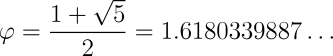
which is found in many aspects of nature and, pleasing to the human eye, commonplace in architecture and design.
The program evaluates the number of terms specified in column 6 of the
store (change the value on the N006 number card at the
top to compute fewer or more terms), and for the second and successive
terms, the ratio of the term to its predecessor to ten decimal places.
You will see the ratio value quickly converge toward φ, the golden
ratio.
![]() Newton's method
(or the Newton-Raphson method) is a numerical technique
for finding roots to real-valued functions by making an
initial guess which is then refined based upon the value
of the function at the guess and its discrepancy with
the value sought. Newton's method is one of the most
fundamental algorithms in numerical computation.
Newton's method
(or the Newton-Raphson method) is a numerical technique
for finding roots to real-valued functions by making an
initial guess which is then refined based upon the value
of the function at the guess and its discrepancy with
the value sought. Newton's method is one of the most
fundamental algorithms in numerical computation.
Here we demonstrate it by evaluating the square root of a number N. We make an initial guess of one half of the number (we could make a closer guess with a more complicated expression, but Newton's method converges so quickly there isn't any reason to go to the trouble), then refine our guess in subsequent iterations through the process:
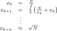
and continue to iterate until the estimation of the square root, x, does not change from one iteration to the next to the precision set for the calculation.
The program takes the square root of the number initially placed in
column 000 of the Store, leaving the result in the same column.
Computation is performed in fixed-point arithmetic, with the number
of decimal places specified by the “A set decimal places”
card at the top of the program. By default, the square root of 2 is
evaluated, but you can compute the square root of any non-negative
number by changing the value on the N000 number card.
The argument, successive approximations for each iteration, and
result are displayed on the Printer. The result computed for the
square root of two to twenty-five decimal places will be
1.4142135623730950488016887. This value would normally be
rounded to one fewer decimal place, yielding the correct
value to twenty-four decimal places of
1.414213562373095048801689. At the end of the computation a
summary of Engine operations and estimate of the time to complete
them is displayed on the Attendant's Log.
![]() The
limaçon, or
limaçon of Pascal, is a quartic curve defined
in Cartesian coordinates as the locus of solutions to
the equation:
The
limaçon, or
limaçon of Pascal, is a quartic curve defined
in Cartesian coordinates as the locus of solutions to
the equation:
(x2 + y2 − ax)2 = b2(x2 + y2)
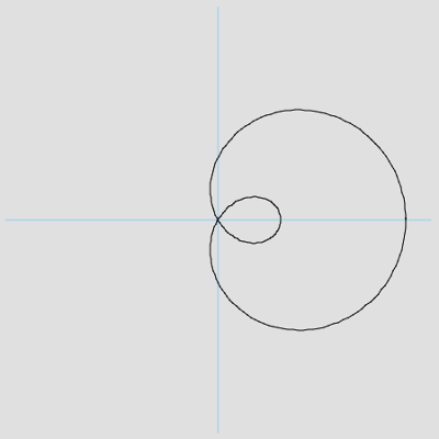
where a and b are parameters which control the size and shape of the curve. Transforming to polar coordinates, the curve may be expressed in parametric form as:
x = (b + a cos t) cos t
y = (b + a cos t) sin t
It is this form which is used in the program, with the parameter varying from 0 to 2π to plot the curve. Calculations are performed with 25 decimal places of precision, using the Mathematical Function Library to evaluate the sine and cosine functions at each iteration. The computation is entirely straightforward and takes no advantage of the curve's symmetry with respect to the x axis. The curve is plotted on the Curve Drawing Apparatus, after first plotting the x and y axes in light blue. At the end of the plot, the Attendant's Log displays the (breathtaking) number of operations performed and how long the Engine might have taken to execute them. Parameters a and b are specified at the top of the program; try varying them to see how they affect the plotted curve.
![]() One of the first problems to which mechanical, electromechanical,
and electronic computers were applied was calculating tables for
naval gunnery and army artillery. Indeed,
ENIAC,
one of the first electronic computers, was funded by the U.S. Army
with that application in mind. The flight of an artillery shell, and
hence how a gun must be aimed for it to hit its target, depends in
a complex manner upon a multitude of factors: the muzzle velocity with
which it leaves the gun, its mass, its size and shape (which determines how much
air resistance it will encounter in flight and the degree wind may
cause it to diverge from a pure ballistic trajectory), the barometric
pressure and humidity of the air through which it is passing, the elevation
of the gun's barrel, and more. Naval gunnery further complicates the
problem, since both the ship from which the gun is fired and the target
may be moving with respect to one another, and pitching and rolling due
to rough seas.
One of the first problems to which mechanical, electromechanical,
and electronic computers were applied was calculating tables for
naval gunnery and army artillery. Indeed,
ENIAC,
one of the first electronic computers, was funded by the U.S. Army
with that application in mind. The flight of an artillery shell, and
hence how a gun must be aimed for it to hit its target, depends in
a complex manner upon a multitude of factors: the muzzle velocity with
which it leaves the gun, its mass, its size and shape (which determines how much
air resistance it will encounter in flight and the degree wind may
cause it to diverge from a pure ballistic trajectory), the barometric
pressure and humidity of the air through which it is passing, the elevation
of the gun's barrel, and more. Naval gunnery further complicates the
problem, since both the ship from which the gun is fired and the target
may be moving with respect to one another, and pitching and rolling due
to rough seas.
So formidable is this problem that in the 20th century naval fire control systems were developed: mechanical or electromechanical analogue computers which could solve the problem in close to real time. Before the advent of such machines, gunners relied upon range tables, compiled by a combination of experiment and manual calculation. Given the importance of naval gunnery to the British Empire, it is almost certain that one of the first tasks for which The Analytical Engine would have been employed was the computation of artillery tables for warships and shore batteries.
Problems such as this are best solved through the process of numerical integration. The flight of the artillery shell is traced along its trajectory from muzzle to target in discrete time steps, with all of the factors affecting its path (momentum, gravitational force, air resistance, etc.) computed at each step. This process is lengthy and tedious to do by hand, but it's ready-made for a computing machine, which can work through the successive steps without human intervention.
This sample program illustrates numerical integration by modeling the trajectory of a projectile fired from a British BL 15 inch Mark I naval gun, which served the Royal Navy from 1915 through 1959, including both World Wars. As a sample program, the computation is much simpler than would have been used to create real artillery tables, but the basic principle of numerical integration is the same.
We start by defining the parameters of the problem, physical constants, and options for the computation as number cards at the top of the program. The following table lists these parameters, giving the symbol by which they are referred to below and the column in the Store into which each is placed. Consistent with the Victorian vintage of The Analytical Engine, these definitions and all calculations in the program will be done in quaint imperial units.
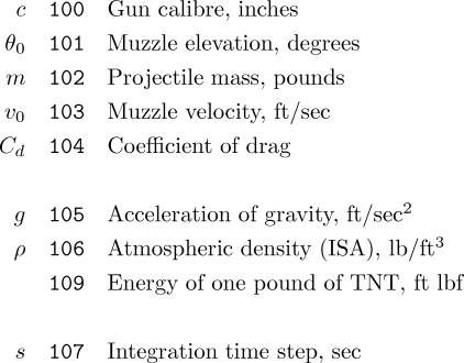
From the calibre (inside barrel diameter) c of the gun, we can calculate the frontal area a of the projectile, which will figure in the calculation of atmospheric drag, from the formula for the area of a circle.
![]()
At each step n in the calculation, we start with the current velocity of the projectile vn, its distance downrange xn, its altitude yn, and the angle of its motion to the horizontal θn. At the start of the computation, these values are initialised with velocity equal to the gun's muzzle velocity, distance and altitude 0, and angle that of the gun's muzzle elevation. In each step, the effects of gravity and air resistance on the projectile will be calculated and used to update these quantities, which are then passed on to the next iteration. The process continues until the altitude goes negative, indicating the projectile has impacted the Earth.
We start by calculating the effect of air resistance, d. This is proportional to the product of the air density ρ, the coefficient of drag Cd (a measure of how the projectile's shape affects the drag it will encounter), the frontal area of the projectile a (computed above), and the square of the projectile's velocity vn2. Drag has the units of force and, acting over the period of the time step s, reduces the projectile's momentum, originally vn m, by the amount d s, giving the new momentum p. Dividing the momentum by the mass of the projectile m gives us its velocity vd as reduced by air resistance. Taking the cosine and sine of this velocity gives the new horizontal vx and vertical vy components of the projectile's velocity.
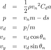
The horizontal and vertical velocity must be treated separately since the acceleration of gravity only acts upon the vertical component of velocity, decreasing it over time s by g s. Taking the square root of the sum of the squares of the horizontal and gravity-affected vertical velocities gives the new velocity vn+1 at the end of the time step, and the arc tangent of the vertical velocity divided by the horizontal velocity gives θn+1, its new angle of motion. Multiplying the horizontal and vertical velocities by the time step and adding them respectively to the range and altitude updates these quantities: xn+1 and yn+1. If the new altitude is negative, the projectile has impacted and we're done. Otherwise, we continue for another step, starting with the updated position, velocity, and angle just computed.
At the end of the computation, a summary appears on the Printer, both with and without the effects of atmospheric drag. The latter is not calculated because the Royal Navy anticipated naval battles on the Moon, but to illustrate the degree air resistance affects the flight of an artillery shell. Try increasing the coefficient of drag on the N104 card to see how it reduces the range and altitude reached by the projectile. A massive projectile moving faster than the speed of sound delivers a large amount of kinetic energy to its target, quite apart from any explosives with which it may have been filled. This kinetic energy is calculated in “foot pounds” (another example of sloppy terminology in imperial units, users of which often fail to make the distinction between weight and mass—the correct term is “foot lbf” where “lbf” stands for “pounds of force”). The energy is then compared to the quantity in pounds of the high explosive TNT which would release the same energy.
     Computation with atmospheric drag

Time of flight: 64.0 seconds
Range: 32030.1 yards
Max altitude: 5439.1 yards
Velocity at impact: 1468.6 ft/sec
Impact kinetic energy: 64957619.1 foot pounds (47.3 pounds of TNT)

     Computation without atmospheric drag

Time of flight: 76.0 seconds
Range: 53926.8 yards
Max altitude: 7416.6 yards
Velocity at impact: 2482.6 ft/sec
Impact kinetic energy: 185629564.4 foot pounds (135.2 pounds of TNT)
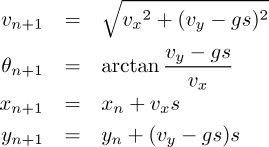
The Curve Drawing Apparatus will display the trajectory of the projectile, both taking into account air resistance (the black curve) and without air resistance (blue curve). Note how increasing the drag coefficient (the N104 number card at the top of the program) affects the trajectory, including deviation from the parabola expected absent the effects of atmospheric drag. With very high drag, the projectile almost comes to a stop and falls from the sky
![]() Once we have a deterministic and high-precision computing device such as
The Analytical Engine, it may seem distinctly odd, if not somewhat
scandalous, to use it to generate random numbers, but there are a number
of applications in mathematics, statistics, and the sciences where
we wish to randomly sample, for example, in computations using the
Monte Carlo method.
Once we have a deterministic and high-precision computing device such as
The Analytical Engine, it may seem distinctly odd, if not somewhat
scandalous, to use it to generate random numbers, but there are a number
of applications in mathematics, statistics, and the sciences where
we wish to randomly sample, for example, in computations using the
Monte Carlo method.
A pseudorandom sequence generator is an algorithm which, although deterministic, produces a sequence of outputs which behave like genuinely random sequences produced through natural processes such as radioactive decay. This program implements and demonstrates a pseudorandom generator which uses two multiplicative congruential generators whose values are combined to increase the period of the results. The generators are “seeded” by a value initially supplied in column 0 of the store when the generator is initialised by including the cards for prand_init from the library; this may be any number between 1 and 2147483647. Subsequently, each time the prand_next cards from the library are executed, a fixed point pseudorandom number between 0 and 1, with the number of decimal places specified by the “A set decimal places to n” card, will be returned in column 0 of the store.
The sample program uses the library cards to generate and print
50 (change the N011 card at the top of the program if you prefer a
different number) pseudorandom values and performs one of the simplest
randomness tests on them: computing their mean value. For a uniformly
distributed sequence of random values between 0 and 1, the mean value
should approach 0.5 as the length of the series increases. The seed
value for the generator is specified by the N000 card
at the top; changing it will produce entirely different values in
the sequence, but have little effect on the mean value. The technique
used to generate the pseudorandom numbers has around 10 decimal places
of precision: nothing will be gained by setting the fixed decimal point
to a larger value.
![]() Now that we have a pseudorandom number generator, let's take it to the
casino and have some fun. Using the generator introduced in the
previous example, it is possible to (very, very slowly) approximate the
value of π.
Now that we have a pseudorandom number generator, let's take it to the
casino and have some fun. Using the generator introduced in the
previous example, it is possible to (very, very slowly) approximate the
value of π.
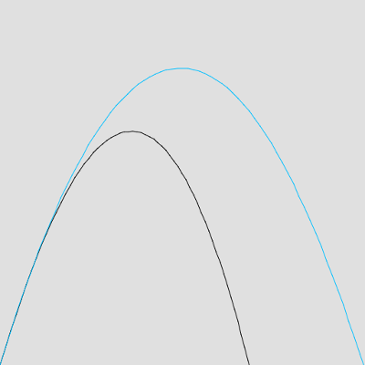
Imagine a square with edges of length l = 2 (which happens to be the shape of the drawing surface of the Engine's Curve Drawing Apparatus). Now inscribe a circle of radius r within this square; we'll draw it with the centre of the circle at the square's centre to simplify the calculations, but it doesn't matter where it's drawn. Now plot a number n of points at random locations within the square and count how many points i fall inside the circle. The area of the circle is a = πr², so the probability any given random point will fall within the circle is p = a/l² = πr²/4. A little algebra lets us solve for π = 4p/r². From a number of random points, we can estimate the probability of points falling within the circle as p ≅ i/n. Finally, we can estimate π ≅ (4 i/n)/r².
The sample program uses the pseudorandom generator to produce random coordinate pairs in the range ±1, determines whether each point falls inside or outside the circle (its radius, 0.5 by default, may be changed by altering the value on the N106 number card at the top), and counts points inside and total points. Periodically (the frequency it set by N120), an estimate for π is calculated as described above and printed along with the number of points generated so far. The circle and points are plotted on the Curve Drawing Apparatus, with points inside the circle in green and those outside blue. The plot is cleared and restarted every 2500 (set by N122) points due to limitations in the implementation of the Curve Drawing Apparatus. Set N150 to 0 to suppress the plotting of points entirely.
Here are the first ten lines output from the program, showing the estimates for the first thousand random points. The first column is the number of random points plotted, the second the estimate of π, and the third the error of the estimate with regard to the correct value.
100:  3.6800000000 17.13%
200:  3.5200000000 12.04%
300:  3.6800000000 17.13%
400:  3.6800000000 17.13%
500:  3.5200000000 12.04%
600:  3.6266666664 15.44%
700:  3.5428571428 12.77%
800:  3.4000000000 8.22%
900:  3.2711111108 4.12%
1000:  3.2160000000 2.36%
As the number of points crosses 30,000, the error in the estimated value has declined substantially. Because this is a random, statistical process and the resolution of the generator and plot are finite, the estimate will continue to oscillate around the correct value as more and more points are plotted.
29700:  3.1380471380 0.11%
29800:  3.1366442952 0.15%
29900:  3.1363210700 0.16%
30000:  3.1365333332 0.16%
30100:  3.1394019932 0.06%
30200:  3.1401324500 0.04%
30300:  3.1419141912 0.01%
30400:  3.1415789472 0.00%
30500:  3.1412459016 0.01%
30600:  3.1393464052 0.07%
Several other documents related to The Analytical Engine contain sample programs. Here are links to them.
![]()