| Two Bits | One Bit | |||
|---|---|---|---|---|
 |
 |
 |
 |
|
| Heads | Tails | Heads | Tails | |
Most experimental searches for paranormal phenomena are statistical in nature. A subject repeatedly attempts a task with a known probability of success due to chance, then the number of actual successes is compared to the chance expectation. If a subject scores consistently higher or lower than the chance expectation after a large number of attempts, one can calculate the probability of such a score due purely to chance, and then argue, if the chance probability is sufficiently small, that the results are evidence for the existence of some mechanism (precognition, telepathy, psychokinesis, cheating, etc.) which allowed the subject to perform better than chance would seem to permit.
Suppose you ask a subject to guess, before it is flipped, whether a coin will land with heads or tails up. Assuming the coin is fair (has the same probability of heads and tails), the chance of guessing correctly is 50%, so you'd expect half the guesses to be correct and half to be wrong. So, if we ask the subject to guess heads or tails for each of 100 coin flips, we'd expect about 50 of the guesses to be correct. Suppose a new subject walks into the lab and manages to guess heads or tails correctly for 60 out of 100 tosses. Evidence of precognition, or perhaps the subject's possessing a telekinetic power which causes the coin to land with the guessed face up? Well,…no. In all likelihood, we've observed nothing more than good luck. The probability of 60 correct guesses out of 100 is about 2.8%, which means that if we do a large number of experiments flipping 100 coins, about every 35 experiments we can expect a score of 60 or better, purely due to chance.
But suppose this subject continues to guess about 60 right out of a hundred, so that after ten runs of 100 tosses—1000 tosses in all, the subject has made 600 correct guesses. The probability of that happening purely by chance is less than one in seven billion, so it's time to start thinking about explanations other than luck. Still, improbable things happen all the time: if you hit a golf ball, the odds it will land on a given blade of grass are millions to one, yet (unless it ends up in the lake or a sand trap) it is certain to land on some blades of grass.
Finally, suppose this “dream subject” continues to guess 60% of the flips correctly, observed by multiple video cameras, under conditions prescribed by skeptics and debunkers, using a coin provided and flipped by The Amazing Randi himself, with a final tally of 1200 correct guesses in 2000 flips. You'd have to try the 2000 flips more than 5×10¹⁸ times before you'd expect that result to occur by chance. If it takes a day to do 2000 guesses and coin flips, it would take more than 1.3×10¹⁶ years of 2000 flips per day before you'd expect to see 1200 correct guesses due to chance. That's more than a million times the age of the universe, so you'd better get started soon!
Claims of evidence for the paranormal are usually based upon statistics which diverge so far from the expectation due to chance that some other mechanism seems necessary to explain the experimental results. To interpret the results of our RetroPsychoKinesis experiments, we'll be using the mathematics of probability and statistics, so it's worth spending some time explaining how we go about quantifying the consequences of chance.
Note to mathematicians: The following discussion of probability is deliberately simplified to consider only binomial and normal distributions with a probability of 0.5, the presumed probability of success in the experiments in question. I decided that presenting and discussing the equations for arbitrary probability would only decrease the probability that readers would persevere and arrive at an understanding of the fundamentals of probability theory.
In slang harking back to the days of gold doubloons and pieces of eight, the United States quarter-dollar coin is nicknamed “two bits”. The Fourmilab radioactive random number generator produces a stream of binary ones and zeroes, or bits. Since we expect the generator to produce ones and zeroes with equal probability, each bit from the generator is equivalent to a coin flip: heads for one and tails for zero. When we run experiments with the generator, in effect, we're flipping a binary coin, one bit—twelve and a half cents!
| Two Bits | One Bit | |||
|---|---|---|---|---|
 |
 |
 |
 |
|
| Heads | Tails | Heads | Tails | |
(We could, of course, have called zero heads and one tails; since both occur with equal probability, the choice is arbitrary.) Each bit produced by the random number generator is a flip of our one-bit coin. Now the key thing to keep in mind about a genuine random number generator or flip of a fair coin is that it has no memory or, as mathematicians say, each bit from the generator or flip is independent. Even if, by chance, the coin has come up heads ten times in a row, the probability of getting heads or tails on the next flip is precisely equal. Gamblers who've seen a coin come up heads ten times in a row may believe “tails is way overdue”, but the coin doesn't know and couldn't care less about the last ten flips; the next flip is just as likely to be the eleventh head in a row as the tail that breaks the streak.
Even though there is no way whatsoever to predict the outcome of the next flip, if we flip a coin a number of times, the laws of probability allow us to predict, with greater accuracy as the number of flips increases, the probability of obtaining various results. In the discussion that follows, we'll ignore the order of the flips and only count how many times the coin came up heads. Since heads is one and tails is zero, we can just add up the results from the flips, or the bits from the random generator.
Suppose we flip a coin four times. Since each flip can come up heads or tails, there are 16 possible outcomes, tabulated below, grouped by the number of heads in the four flips.
| Number of Heads |
Results of Flips | Number of Ways |
|---|---|---|
| 0 | 1 | |
| 1 |
|
4 |
| 2 |
|
6 |
| 3 |
|
4 |
| 4 | 1 |
Number of Ways summarises how many different ways the results of the four flips could end up with a given number of heads. Since the only way to get zero heads is for all four flips to be tails, there's only one way that can occur. One head out of four flips can happen four different ways since each of the four flips could have been the head. Two heads out of four flips can happen six different ways, as tabulated. And since what's true of heads applies equally to tails, there are four ways to get three heads and one way to get four.
Mathematically, the number of ways to get x heads (or tails) in n flips is spoken of as the “number of combinations of n things taken x at a time”, which is written as:

This, it turns out, can be calculated for any positive integers n and x whatsoever, as follows.

For example, if we plug in 4 for n and 2 for x, we get
as expected. Plotting the number of ways we can get different numbers of heads yields the following graph.
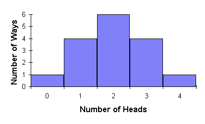
Since the coin is fair, each flip has an equal chance of coming up heads or tails, so all 16 possible outcomes tabulated above are equally probable. But since there are 6 ways to get 2 heads, in four flips the probability of two heads is greater than that of any other result. We express probability as a number between 0 and 1. A probability of zero is a result which cannot ever occur: the probability of getting five heads in four flips is zero. A probability of one represents certainty: if you flip a coin, the probability you'll get heads or tails is one (assuming it can't land on the rim, fall into a black hole, or some such).
The probability of getting a given number of heads from four flips is, then, simply the number of ways that number of heads can occur, divided by the number of total results of four flips, 16. We can then tabulate the probabilities as follows.
| Number of Heads |
Number of Ways |
Probability |
|---|---|---|
| 0 | 1 | 1/16 = 0.0625 |
| 1 | 4 | 4/16 = 0.25 |
| 2 | 6 | 6/16 = 0.375 |
| 3 | 4 | 4/16 = 0.25 |
| 4 | 1 | 1/16 = 0.0625 |
Since we are absolutely certain the number of heads we get in four flips is going to be between zero and four, the probabilities of the different numbers of heads should add up to 1. Summing the probabilities in the table confirms this. Further, we can calculate the probability of any collection of results by adding the individual probabilities of each. Suppose we'd like to know the probability of getting fewer than three heads from four flips. There are three ways this can happen: zero, one, or two heads. The probability of fewer than three, then, is the sum of the probabilities of these results, 1/16 + 4/16 + 6/16 = 11/16 = 0.6875, or a little more than two out of three. So to calculate the probability of one outcome or another, sum the probabilities.
To get probability of one result and another from two separate experiments, multiply the individual probabilities. The probability of getting one head in four flips is 4/16 = 1/4 = 0.25. What's the probability of getting one head in each of two successive sets of four flips? Well, it's just 1/4 × 1/4 = 1/16 = 0.0625.
The probability for any number of heads x in any number of flips n is thus:
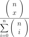
the number of ways in which x heads can occur in n flips, divided by the number of different possible results of the series of flips, measured by number of heads. But there's no need to sum the combinations in the denominator, since the number of possible results is simply two raised to the power of the number of flips. So, we can simplify the expression for the probability to:

Let's see how the probability behaves as we make more and more flips. Since we have a general formula for calculating the probability for any number of heads in any number of flips, we can graph of the probability for various numbers of flips.
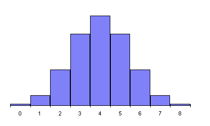
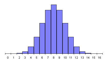
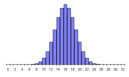
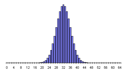
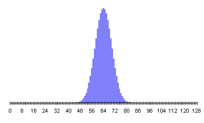
In every case, the peak probability is at half the number of flips and declines on both sides, more steeply as the number of flips increases. This is the simple consequence of there being many more possible ways for results close to half heads and tails to occur than ways that result in a substantial majority of heads or tails. The RPKP experiments involve a sequence of 1024 random bits, in which the most probable results form a narrow curve centred at 512. A document giving probabilities for results of 1024 bit experiments with chance expectations greater than one in 100 thousand million runs is available, as is a much larger table listing probabilities for all possible results. (The latter document is more than 150K bytes and will take a while to download, and contains a very large table which some Web browsers, particularly on machines with limited memory, may not display properly.)
As we make more and more flips, the graph of the probability of a given number of heads becomes smoother and approaches the “bell curve”, or normal distribution, as a limit. The normal distribution gives the probability for x heads in n flips as:

where μ=n/2 and σ is the standard deviation, a measure of the breadth of the curve which, for equal probability coin flipping, is:
We keep the standard deviation separate, as opposed to merging it into the normal distribution probability equation, because it will play an important rôle in interpreting the results of our experiments. To show how closely the probability chart approaches the normal distribution even for a relatively small number of flips, here's the normal distribution plotted in red, with the actual probabilities for number of heads in 128 flips shown as blue bars.
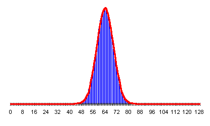
The probability the outcome of an experiment with a sufficiently large number of trials is due to chance can be calculated directly from the result, and the mean and standard deviation for the number of trials in the experiment. For additional details, including an interactive probability calculator, please visit the z Score Probability Calculator.
This is all very persuasive, you might say, and the formulas are suitably intimidating, but does the real world actually behave this way? Well, as a matter of fact, it does, as we can see from a simple experiment. Get a coin, flip it 32 times, and write down the number of times heads came up. Now repeat the experiment fifty thousand times. When you're done, make a graph of the number of 32-flip sets which resulted in a given number of heads. Hmmmm…32 times 50,000 is 1.6 million, so if you flip the coin once a second, twenty-four hours per day, it'll take eighteen and a half days to complete the experiment….
Instead of marathon coin-flipping, let's use the same HotBits hardware random number generator our experiments employ. It's a simple matter of programming to withdraw 1.6 million bits from the generator, divide them up into 50,000 sets of 32 bits each, then compute a histogram of the number of sets containing each possible number of one bits (heads). The results from this experiment are presented in the following graph.
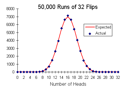
The red curve is the number of runs expected to result in each value of heads, which is simply the probability of that number of heads multiplied by the total number of experimental runs, 50,000. The blue diamonds are the actual number of 32 bit sets observed to contain each number of one bits. It is evident that the experimental results closely match the expectation from probability. Just as the probability curve approaches the normal distribution for large numbers of runs, experimental results from a truly random source will inexorably converge on the predictions of probability as the number of runs increases.
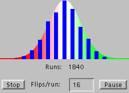 If
your Web browser supports Java
applets, our Probability Pipe
Organ lets you run interactive experiments which demonstrate how
the results from random data approach the normal
curve expectation as the number of experiments grows large.
Performing an experiment amounts to asking the Universe a question. For the answer, the experimental results, to be of any use, you have to be absolutely sure you've phrased the question correctly. When searching for elusive effects among a sea of random events by statistical means, whether in particle physics or parapsychology, one must take care to apply statistics properly to the events being studied. Misinterpreting genuine experimental results yields errors just as serious as those due to faults in the design of the experiment.
Evidence for the existence of a phenomenon must be significant, persistent, and consistent. Statistical analysis can never entirely rule out the possibility that the results of an experiment were entirely due to chance—it can only calculate the probability of occurrence by chance. Only as more and more experiments are performed, which reproduce the supposed effect and, by doing so, further decrease the probability of chance, does the evidence for the effect become persuasive.
To show how essential it is to ask the right question, consider an experiment in which the subject attempts to influence a device which generates random digits from 0 to 9 so that more nines are generated than expected by chance. Each experiment involves generation of one thousand random digits. We run the first experiment and get the following result:
51866599999944246273322297520235159670265786865762
83920280286669261956417760577150505375232340788171
46551582885930322064856497482202377988394190796683
36456436836261696793837370744918197880364326675561
63557778635028561881986962010589509079505189756148
71722255387675577937985730026325400514696800042830
49134963200862681703176774115437941755363670637799
08279963556956436572800286835535562483733337524409
90735067709628443287363500729444640394058938260556
35615446832321914949835991535024593960198026143550
34915341561413975080553492042984685869042671369729
59432799270157302860632198198519187171162147204313
26736371990032510981560378617615838239495314260376
28555369005714414623002367202494786935979014596272
75647327983564900896013913125375709712947237682165
84273385694198868267789456099371827798546039550481
93966363733020953807261965658687028741391908959254
79109139065222171490342469937003707021339710682734
97173738046984452113756225260095828324586288486644
14887777251716547950457638477301077505585332159232
The digit frequencies from this run are:
| Digit | Occurrences |
|---|---|
| 0 | 94 |
| 1 | 81 |
| 2 | 96 |
| 3 | 111 |
| 4 | 84 |
| 5 | 111 |
| 6 | 111 |
| 7 | 112 |
| 8 | 91 |
| 9 | 109 |
There's no obvious evidence for a significant excess of nines here (we'll see how to calculate this numerically before long). There was an excess of nines over the chance expectation, 100, but greater excesses occurred for the digits 3, 5, 6, and 7. But take a look at the first line of the results!
    51866599999944246273322297520235159670265786865762
                            .
                            .
                            .
These digits were supposed to be random, yet in the first thousand, the first dozen for that matter, we found a pattern as striking as “999999”. What's the probability of that happening? Just the number of possible numbers of d digits which contain one or more sequences of p or more consecutive nines:

Plugging in 1000 for d and 6 for p yields:

So the probability of finding “999999” in a set of 1000 random digits is less than one in a thousand! So then, are the digits not random, after all? Might our subject, while failing to influence the outcome of the experiment in the way we've requested, have somehow marked the results with a signature of a thousand-to-one probability of appearing by chance? Or have we simply asked the wrong question and gotten a perfectly accurate answer that doesn't mean what we think it does at first glance?
The latter turns out to be the case. The data are right before our eyes, and the probability we calculated is correct, but we asked the wrong question, and in doing so fell into a trap littered with the bones of many a naïve researcher. Note the order in which we did things. We ran the experiment, examined the data, found something seemingly odd in it, then calculated the probability of that particular oddity appearing by chance. We asked the question, “What is the probability of ‘999999’ appearing in a 1000 digit random sequence?” and got the answer “less than one in a thousand”, a result most people would consider significant. But since we calculated the probability after seeing the data, in fact we were asking the question “What is the chance that ‘999999’ appears in a 1000 digit random sequence which contains one occurrence of ‘999999’?”. The answer to that question is, of course, “certainty”.
In the original examination of the data, we were really asking “What is the probability we'll find some striking sequence of six digits in a random 1000 digit number?”. We can't precisely quantify that without defining what “striking” means to the observer, but it is clearly quite high. Consider that I could have made the case just as strongly for “000000”, “777777” or any other six-digit repeat. That alone reduces the probability of occurrence by chance to one in ten. Or, perhaps I might have pointed out a run of digits like “123456”, “012345”, “987654”, and so on; or the first five or six digits of a mathematical constant such as Pi, e, or the square root of two; regular patterns like “101010”, “123321”, or a multitude of others; or maybe my telephone or license plate number, or the subject's! It is, in fact, very likely you'll find some pattern you consider striking in a random 1000-digit number.
But, of course, if you don't examine the data from an experiment, how are you going to notice if there's something odd about it? Now we'll see how a hypothesis is framed, tested by a series of experiments, and confirmed or rejected by statistical analysis of the results. So, let's pursue this a bit further, exploring how we frame a hypothesis based on an observation, run experiments to test it, and then analyse the results to determine whether they confirm or deny the hypothesis, and to what degree of certainty.
Our observation, based on examining the first thousand random digits, is that “999999” appears once, while the probability of “999999” appearing in a randomly chosen 1000 digit number is less than one in a thousand. Based on this observation we then suggest:
Hypothesis: The sequence “999999” appears more frequently in 1000-digit sequences with the subject attempting to influence the generator than would be expected by chance.
We can now proceed to test this experimentally. If the sequence “999999” has a probability of occurring in a 1000 digit sequence of 0.000995, then for a thousand consecutive 1000 digit sequences (a million digits in all), the probability of “999999” appearing will be 0.995, almost unity. (To be correct, it's important to test each 1000 digit sequence separately, then sum the results for 1000 consecutive sequences. If we were to scan all million digits as one sequence, we would count cases where the sequence “999999” begins in one 1000 digit sequence and ends in the next. The probability (which you can calculate from the equation above) of finding “999999” in a million digit sequence is 0.999995, somewhat higher than the 0.995 with the million digits are treated as separate 1000 digit experiments.)
We will perform, then, the following experiment. With our ever-patient subject continuing to attempt to influence the output of the generator, we will produce a million more sequences of 1000 digits and, in each, count occurrences of “999999”. Every 1000 sequences, we'll record the number of occurrences, repeating the process until we've generated a thousand runs of a million digits—109 digits in all. With that data in hand, we'll see whether the “999999 effect” is genuine or a fluke attributable to chance.
Here is a plot of the number of occurrences of the sequence “999999” per block of 1000 digits over the thousand repetitions of the thousand sequence experiment. The number of occurrences expected by chance, 0.995, is marked by the green line.
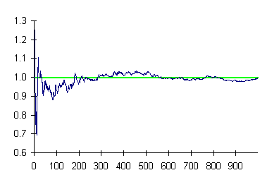
At the outset, the results diverged substantially from chance, as is frequently the case for small sample sizes. But as the number of experiments increased, the results converged toward the chance expectation, ending up in a decreasing magnitude random walk around it. This is precisely what is expected from probability theory, and hence we conclude no “999999 effect” exists.
So far, we've seen how the laws of probability predict the outcome of large numbers of experiments involving random data, how to calculate the probability of a given experimental result being due to chance, and how one goes about framing a hypothesis, then designing and running a series of experiments to test it. Now it's time to examine how to analyse the results from the experiments to determine whether they provide evidence for the hypothesis and, if so, how much.
Since its introduction in 1900 by Karl Pearson, the chi-square (X²) test has become the most widely used measure of the significance to which experimental results support or refute a hypothesis. Applicable to any experiment where discrete results can be measured, it is used in almost every field of science. The chi-square test is the final step in a process which usually proceeds as follows.
No experiment or series of experiments can ever prove a hypothesis; one can only rule out other hypotheses and provide evidence that assuming the truth of the hypothesis better explains the experimental results than discarding it. In many fields of science, the task of estimating the null-hypothesis results can be formidable, and can lead to prolonged and intricate arguments about the assumptions involved. Experiments must be carefully designed to exclude selection effects which might bias the data.
Fortunately, retropsychokinesis experiments have an easily stated and readily calculated null hypothesis: “The results will obey the statistics for a sequence of random bits.” The fact that the data are prerecorded guarantees (assuming the experiment software is properly implemented and the results are presented without selection or modification) that run selection or other forms of cheating cannot occur. (Anybody can score better than chance at coin flipping if they're allowed to throw away experiments that come out poorly!) Finally, the availability of all the programs in source code form and the ability of others to repeat the experiments on their own premises will allow independent confirmation of the results obtained here.
So, as the final step in analysing the results of a collection of n experiments, each with k possible outcomes, we apply the chi-square test to compare the actual results with the results expected by chance, which are just, for each outcome, its probability times the number of experiments n.
Mathematically, the chi-square statistic for an experiment with k possible outcomes, performed n times, in which Y1, Y2,… Yk are the number of experiments which resulted in each possible outcome, where the probabilities of each outcome are p1, p2,… pk is:

It's evident from examining this equation that the closer the measured values are to those expected, the lower the chi-square sum will be. Further, from a chi-square sum, the probability Q that the X² sum for an experiment with d degrees of freedom (where d=k−1, one less the number of possible outcomes) is consistent with the null hypothesis can be calculated as:

Where Γ is the generalisation of the factorial function to real and complex arguments:
![]()
Unfortunately, there is no closed form solution for Q, so it must be evaluated numerically. If your Web browser supports JavaScript, you can use the Chi-Square Calculator to calculate the probability from a chi-square value and number of possible outcomes, or calculate the chi-square from the probability and the number of possible outcomes.
In applying the chi-square test, it's essential to understand that only very small probabilities of the null hypothesis are significant. If the probability that the null hypothesis can explain the experimental results is above 1%, an experiment is generally not considered evidence of a different hypothesis. The chi-square test takes into account neither the number of experiments performed nor the probability distribution of the expected outcomes; it is valid only as the number of experiments becomes large, resulting in substantial numbers for the most probable results. If a hypothesis is valid, the chi-square probability should converge on a small value as more and more experiments are run.
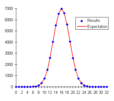
Now let's examine an example of how the chi-square test identifies experimental results which support or refute a hypothesis. Our simulated experiment consists of 50,000 runs of 32 random bits each. The subject attempts to influence the random number generator to emit an excess of one or zero bits compared to the chance expectation of equal numbers of zeroes and ones. The following table gives the result of a control run using the random number generator without the subject's attempting to influence it. Even if the probability of various outcomes is easily calculated, it's important to run control experiments to make sure there are no errors in the experimental protocol or apparatus which might bias the results away from those expected. The table below gives, for each possible number of one bits, the number of runs which resulted in that count, the expectation from probability, and the corresponding term in the chi-square sum. The chi-square sum for the experiment is given at the bottom.
| Control Run | |||
|---|---|---|---|
 | |||
| Ones | Results | Expectation | X² Term |
| 0 | 0 | 1.16×10⁻⁵ | 1.16×10⁻⁵ |
| 1 | 0 | 0.000372529 | 0.000372529 |
| 2 | 0 | 0.0057742 | 0.0057742 |
| 3 | 0 | 0.057742 | 0.057742 |
| 4 | 0 | 0.418629 | 0.418629 |
| 5 | 3 | 2.34433 | 0.183383 |
| 6 | 15 | 10.5495 | 1.87756 |
| 7 | 27 | 39.1837 | 3.78839 |
| 8 | 124 | 122.449 | 0.0196425 |
| 9 | 340 | 326.531 | 0.555579 |
| 10 | 764 | 751.021 | 0.224289 |
| 11 | 1520 | 1502.04 | 0.214686 |
| 12 | 2598 | 2628.57 | 0.355633 |
| 13 | 4017 | 4043.96 | 0.179748 |
| 14 | 5506 | 5488.23 | 0.0575188 |
| 15 | 6523 | 6585.88 | 0.600345 |
| 16 | 6969 | 6997.5 | 0.11605 |
| 17 | 6581 | 6585.88 | 0.00361487 |
| 18 | 5586 | 5488.23 | 1.74162 |
| 19 | 4057 | 4043.96 | 0.0420422 |
| 20 | 2570 | 2628.57 | 1.30526 |
| 21 | 1531 | 1502.04 | 0.558259 |
| 22 | 749 | 751.021 | 0.00544023 |
| 23 | 345 | 326.531 | 1.04463 |
| 24 | 126 | 122.449 | 0.102971 |
| 25 | 41 | 39.1837 | 0.0841898 |
| 26 | 6 | 10.5495 | 1.96196 |
| 27 | 0 | 2.34433 | 2.34433 |
| 28 | 2 | 0.418629 | 5.97362 |
| 29 | 0 | 0.057742 | 0.057742 |
| 30 | 0 | 0.0057742 | 0.0057742 |
| 31 | 0 | 0.000372529 | 0.000372529 |
| 32 | 0 | 1.16×10⁻⁵ | 1.16×10⁻⁵ |
| X² Sum | 23.8872 | ||
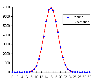
Entering the X² sum of 23.8872 and the degrees of freedom (32, one less than the 33 possible outcomes of the experiment) into the Chi-Square Calculator gives a probability of 0.85. This falls within the “fat region” of the probability curve, and thus supports the null hypothesis, just as we expected.
Next, we invite our subject to attempt to influence the random output of our generator. How? Hypotheses non fingo. Let's just presume that by some means: telekinesis, voodoo, tampering with the apparatus when we weren't looking—whatever, our subject is able to bias the generator so that out of every 200 bits there's an average of 101 one bits and 99 zeroes. This seemingly subtle bias would result in an experiment like the following.
| Run with Subject | |||
|---|---|---|---|
 | |||
| Ones | Results | Expectation | X² Term |
| 0 | 0 | 1.16×10⁻⁵ | 1.16×10⁻⁵ |
| 1 | 0 | 0.000372529 | 0.000372529 |
| 2 | 0 | 0.0057742 | 0.0057742 |
| 3 | 0 | 0.057742 | 0.057742 |
| 4 | 1 | 0.418629 | 0.807377 |
| 5 | 2 | 2.34433 | 0.0505731 |
| 6 | 13 | 10.5495 | 0.569236 |
| 7 | 23 | 39.1837 | 6.68423 |
| 8 | 93 | 122.449 | 7.08254 |
| 9 | 335 | 326.531 | 0.219654 |
| 10 | 705 | 751.021 | 2.82011 |
| 11 | 1424 | 1502.04 | 4.05491 |
| 12 | 2491 | 2628.57 | 7.20039 |
| 13 | 3810 | 4043.96 | 13.5357 |
| 14 | 5480 | 5488.23 | 0.0123496 |
| 15 | 6699 | 6585.88 | 1.94299 |
| 16 | 6871 | 6997.5 | 2.28673 |
| 17 | 6639 | 6585.88 | 0.428464 |
| 18 | 5449 | 5488.23 | 0.280456 |
| 19 | 4298 | 4043.96 | 15.9586 |
| 20 | 2692 | 2628.57 | 1.5304 |
| 21 | 1614 | 1502.04 | 8.34494 |
| 22 | 795 | 751.021 | 2.57533 |
| 23 | 347 | 326.531 | 1.28312 |
| 24 | 150 | 122.449 | 6.19891 |
| 25 | 51 | 39.1837 | 3.56333 |
| 26 | 14 | 10.5495 | 1.12861 |
| 27 | 3 | 2.34433 | 0.183383 |
| 28 | 1 | 0.418629 | 0.807377 |
| 29 | 0 | 0.057742 | 0.057742 |
| 30 | 0 | 0.0057742 | 0.0057742 |
| 31 | 0 | 0.000372529 | 0.000372529 |
| 32 | 0 | 1.16×10⁻⁵ | 1.16×10⁻⁵ |
| X² Sum | 89.6775 | ||
The graph of the result versus the expectation doesn't show any terribly obvious divergence from the expectation, yet the chi-square test unambiguously fingers the bias. A X² sum of 89.6775 in an experiment with 33 possible outcomes (32 degrees of freedom) has a probability of occurring by chance of 0.00000022—about two in ten million—a highly significant result, worthy of follow-up experiments and investigation of possible mechanisms which might explain the deviation from chance.
|
Click on titles to order books on-line from
|
 RetroPsychoKinesis Project Home